Photonics2D#

Version	0
Design space	`Box(0.0, 1.0, (120, 120), float64)`
Objectives	total_overlap: ↑
Conditions	lambda1: 1.5 lambda2: 1.3 blur_radius: 2
Dataset	IDEALLab/photonics_2d_120_120_v0
Import	`from engibench.problems.photonics2d.v0 import Photonics2D`

Photonic Inverse Design 2D Problem (Wavelength Demultiplexer).

Problem Description#

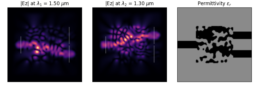
Optimize a 2D material distribution (rho) to function as a wavelength demultiplexer, routing wave with lambda1 to output 1 and lambda2 to output 2. The design variables represent material density that is converted to permittivity using filtering and projection.

Motivation#

The optimization of photonic circuits in general, and multiplexers in particular, was one of the initial and most widely studied problems in the inverse design of electromagnetic/optical devices. In part, this is because multiplexer devices have several interesting properties that make them more difficult to create generative models of, compared to other problems in EngiBench. This includes the fact that, due to the wave properties of the physical phenomena there are usually multiple solutions with equivalent or similar performance, which results from shifting or inverting the phase profile of the electromagnetic wave. This adds complexity to the generative model in that the solution may not have a single unique global minimum. Another motivating factor for including this problem is the complexity of the structures/designs themselves: unlike in structural or thermal compliance problems, which lead to connected structures, the photonics solutions often involve several disconnected elements whose relative position and spacing is governed by the specific wavelengths it needs to demultiplex. This is a difficult prediction and generation task, compared to, e.g., generating a connected beam structure. Thus, it acts as a good counterpoint to add to the library and provides a mechanism to benchmark generative algorithms that can perform well on both connected and disconnected design topologies.

Design space#

This problem simulates a wavelength demultiplexer where the optimized device will direct an electromagnetic wave to one of two possible output ports depending on the wavelength/frequency of the incoming wave. Specifically, the demultiplexer targets two specific wavelengths (referred to \(\lambda_1\) and \(\lambda_2\) in the library), and the performance of the device is how well it can bend or direct the energy toward two specific locations in the device, as measured by how much of the electric field of each wavelength overlaps with the desired output port locations. The design space consists of a 2D array representing the presence of either a high or low permittivity, parameterized by nelx and nely, i.e., \(\text{design_space} = [0,1]^{\text{nelx}\times \text{nely}}\). By default, the library uses a \(120 \times 120\) space, however, this can be modified to non-square design spaces by the user. Specifically, we use a 2D tensor rho (num_elems_x, num_elems_y) with values in [0, 1], representing material density. This is stored as design_space (gymnasium.spaces.Box).

Objectives#

The main objective is to maximize the overlap of the electric field of the simulated wavelength at the target output location, with an optional penalty for the amount of material used (this penalty weight is set to a small default value (\(1e^{-2}\)) for consistency, but can be altered for advanced usage): 0. total_overlap: Objective to maximize, defined as overlap1 * overlap2. Higher is better. This corresponds to the overlap in the target electrical fields with the desired demultiplexing locations. Note that bot simulate and optimize subtract a small material penalty (total_overlap - penalty) to avoid multiple equivalent local optima, but this penalty is small relative to the overlap objective.

Conditions#

These are designed as user-configurable parameters that alter the problem definition. The conditions consist of the two input wavelengths to be demultiplexed – \(\lambda_1\) and \(\lambda_2\), as well as a desired blur_radius (\(r_{blur}\)) parameter, which blurs (using a circular convolution) the pixelized design field for a chosen number of integer pixels\textemdash this blurring essentially creates a penalty on the minimum feature size of the design. The size of the device – expressed as nelx and nely – is also adjustable, and could be viewed as a possible condition for multi-resolution problems, but in practice, as with Beams2D, this is built into the problem definition since it produces a different dataset.

Default problem parameters that can be overridden via the config dict:

lambda1: The first input wavelength in μm (default: 1.5 μm).
lambda2: The first input wavelength in μm (default: 1.3 μm).
blur_radius: Radius for the density blurring filter (default: 2). Higher values correspond to larger elements, which could possibly be more manufacturable.
num_elems_x: Number of grid cells in x (default: 120).
num_elems_y: Number of grid cells in y (default: 120).

In practice, for the dataset loading, we will keep num_elems_x and num_elems_yto set values for each dataset, such that different resolutions correspond to different independent datasets.

Optimization Parameters#

Note: These are advanced parameters that alter the optimization process – we do not recommend changing these if you are only using the library for benchmarking, as it could make results less reproducible across papers using this problem.)

num_optimization_steps: Total number of optimization steps (default: 300).
step_size: Adam optimizer step size (default: 1e-1).
penalty_weight: Weight for the L2 penalty term (default: 1e-2). Larger values reduce unnecessary material, but may lead to worse performance if too large.
eta: Projection center parameter (default: 0.5). There is little reason to change this.
N_proj: Number of projection applications (default: 1). Increasing this can help make the design more binary.
N_blur: Number of blur applications (default: 1). Increasing this smooths the design more.
initial_beta: Initial beta for the optimization continuation scheme (default: 1.0).
save_frame_interval: Interval for saving intermediate design frames during optimization. If > 0, saves a frame every save_frame_interval iterations to the opt_frames/ directory. Default is 0 (disabled).

Internal Constants#

Note: These are not typically changed by users, but provided here for technical reference

dl: Spatial resolution (meters) (default: 40e-9).
Npml: Number of PML cells (default: 20).
epsr_min: Minimum relative permittivity (default: 1.0).
epsr_max: Maximum relative permittivity (default: 12.0).
space_slice: Extra space for source/probe slices (pixels) (default: 8).

Simulator#

The simulation uses the ceviche library’s Finite Difference Frequency Domain (FDFD) solver (fdfd_ez). Optimization uses ceviche.optimizers.adam_optimize with gradients computed via automatic differentiation (autograd). The simulation code uses the \texttt{ceviche} library and specifically, the wave demultiplexer demonstration case provided by the [library authors](https://github.com/fancompute/workshop-invdesign/blob/master/04_Invdes_wdm_scheduling.ipynb} based on their related publication, which uses a similar formalism to an earlier demultiplexer paper by Piggott (2015). The optimization method is first-order and uses the Adam optimizer. Beyond the baseline implementation already available via ceviche, we implemented a polynomial \(\beta\) continuation scheme that performed more reliably than the step-wise continuation scheme used in the original implementation, and EngiBench also possesses the ability to change the starting and ending continuation values, for future research cases where one wishes to estimate or optimize the continuation schedule themselves. Other than these changes, the implementation of this problem is as consistent as possible with that of the original ceviche library.

Dataset#

This problem offers a single datasets of nelx=120 and nely=120, although various sizes of nelx and nely could be generated from the library if desired. The dataset includes columns for the optimal design, all conditions listed above, and the corresponding objective value history as the optimizer optimized toward the optimal design provided in the dataset. The dataset was generated by sampling by sampling at random \(\lambda_1\), \(\lambda_2\) and \(r_{blur}\) over the conditions mentioned above. The dataset is available on the Hugging Face Datasets Hub.

v0#

Fields#

Each dataset contains:

lambda1: The first input wavelength in μm.
lambda2: The second input wavelength in μm.
blur_radius: Radius for the density blurring filter (pixels).
optimal_design: The optimal design density array (shape num_elems_x, num_elems_y).
optimization_history: A list of objective values from the optimization process (field overlap minus penalty, where higher is better) – This is for advanced use.

Creation Method#

To generate a dataset for training, we generate (randomly, uniformly) swept over the following parameters:

\(\lambda_1 \in [0.5\mu m, 1.25\mu m]\) = lambda1 = rng.uniform(low=0.5, high=1.25, size=20) – This corresponds roughly to a portion of the visible spectrum up to near-infrared.
\(\lambda_2 \in [0.75\mu m, 1.5\mu m]\) = lambda2 = rng.uniform(low=0.75, high=1.5, size=20) – This corresponds roughly to a portion of the visible spectrum up to near-infrared.
\(r_{blur}\) = blur_radius = range(0, 5)

Citation#

This problem is directly refactored from the Ceviche Library: https://github.com/fancompute/ceviche and if you use this problem your experiments, you can use the citation below provided by the original library authors:

@article{hughes2019forward,
    title={Forward-Mode Differentiation of Maxwell's Equations},
    author={Hughes, Tyler W and Williamson, Ian AD and Minkov, Momchil and Fan, Shanhui},
    journal={ACS Photonics},
    volume={6},
    number={11},
    pages={3010--3016},
    year={2019},
    publisher={ACS Publications}
}

Lead#

Mark Fuge @markfuge

Photonics2D

Contents