MTO2D

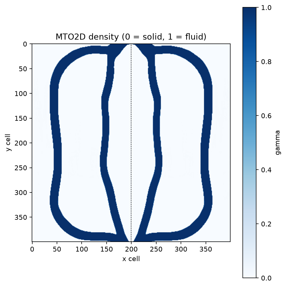
OpenFOAM-based 2D thermofluid topology optimization.

A design is the non-redundant, visually oriented (400, 200) fluid-density half-domain. gamma=0 is solid and gamma=1 is fluid. The right half is implied by symmetry and is created only for rendering.

The built-in optimizer minimizes mean temperature with MMA while treating fluid volume and power dissipation as constraints. Power dissipation is nevertheless exposed as a second EngiBench objective for Pareto analysis.

Version	0
Design space	Box(0.0, 1.0, (400, 200), float32)
Objectives	mean_temperature: ↓ power_dissipation: ↓
Conditions	inlet_velocity: Signed inlet y-velocity in m/s; the nominal dataset range is [-0.095, -0.025]. max_power_dissipation: Dimensionless normalized power-dissipation bound. The retained solver divides physical dissipation by its exact ``D_normalization = 1.57572e-7``. The paper denotes the rounded reference scale ``J1 ≈ 1.58e-7``. The nominal dataset range is [47.7, 75]. The second sweep targeted [50, 75], but 17 of the 5,666 retained rows fall below 50. volfrac: Maximum all-cell fluid volume fraction.
Dataset	IDEALLab/mto_2d_v0
Container	ghcr.io/ideallab/engibench-mto2d@sha256:2887a5c8eaa3fba2d2738188757aeb66fe69d8ef7060698cb8512252aacaa131
Import	from engibench.problems.mto2d.v0 import MTO2D
Lead	Arthur Drake @arthurdrake1

Motivation

Multiphysics topology optimization (MTO) couples fluid flow, heat transfer, and design sensitivities in a single optimization loop, making it one of the most expensive problem families in density-based topology optimization. MTO2D distributes fluid and solid material inside a two-dimensional heat sink so that coolant entering at the top carries heat out at the bottom. Each cold-start optimization solves the incompressible Navier–Stokes and energy-balance equations with adjoint sensitivities for 200 iterations, which is why this problem is a strong benchmark for surrogate and generative approaches that try to warm-start or replace the solver.

The problem, solver, and dataset follow the VQGAN-for-MTO study by Drake et al., which generated thousands of optimized heat sinks over a range of inlet velocities, power-dissipation limits, and fluid volume fractions.

Problem setup

MTO2D models one symmetric half of a water-cooled rectangular heat sink. Coolant enters through a channel at the top, flows through channels placed by the optimizer, and leaves through a channel at the bottom. The paper uses a 10 mm design-domain length, a 2 mm inlet scale, and a uniform heat source of 1e8 W/m².

The inlet has fixed velocity and reference temperature (T = 0). The outlet has zero pressure and no normal temperature gradient. The remaining outer walls are no-slip and adiabatic, and the centerline is a symmetry boundary. For every proposed material layout, the solver computes steady incompressible flow and heat transfer.

Design space

A design is a float32 array with shape (400, 200) and values in [0, 1], storing the non-redundant left half of the symmetric design domain:

• gamma = 0 means solid material.

• gamma = 1 means fluid.

• render() mirrors the half-domain horizontally into a symmetric (400, 400) image.

The example above is a mirrored 400 x 400 rendering of public dataset row train[1977] (volfrac = 0.26), selected for its sparse, smooth fluid channels.

The underlying OpenFOAM field has 86,400 cells: the first 80,000 encode the (400, 200) design in two solver-specific mesh blocks, and the remaining 6,400 are fixed fluid cells (inlet and outlet channels) copied unchanged from the case template. The design_io module owns this mapping so that simulation never silently resizes a design.

Datasets store optimal_design as a flat list<float32> of length 80,000 in C order, following the Beams3D Hub convention; random_design() reshapes rows back to the native (400, 200) representation.

The earlier IDEALLab/MTO-2D NumPy dataset stores each design as a (256, 256) image of the whole left half-domain, produced by a lossy anisotropic bicubic resize of the native field. MTO2D v0 deliberately accepts only the native representation so simulation never silently resizes a topology.

Objectives

EngiBench minimizes both reported objectives, in this order:

0. mean_temperature: mean temperature over the domain, reported in degrees Celsius.

1. power_dissipation: measured fluid power dissipation, reported as the factor J/J1.

The native MMA formulation uses mean temperature as its scalar objective and enforces fluid volume and J < J̄ as constraints. EngiBench also exposes the measured J as a second objective so designs can be compared on a Pareto front. The condition max_power_dissipation is the input bound J̄/J1, not the measured objective. Because that constraint depends on simulation output, simulate_verbose() reports its relative residual as power_dissipation / max_power_dissipation - 1.

Conditions

• inlet_velocity: Signed inlet y-velocity in m/s; the nominal dataset range is [-0.095, -0.025].

• max_power_dissipation: Dimensionless normalized power-dissipation bound. The retained solver divides physical dissipation by its exact ``D_normalization = 1.57572e-7``. The paper denotes the rounded reference scale ``J1 ≈ 1.58e-7``. The nominal dataset range is [47.7, 75]. The second sweep targeted [50, 75], but 17 of the 5,666 retained rows fall below 50.

• volfrac: Maximum all-cell fluid volume fraction.

• inlet_velocity: signed inlet velocity, nominally from -0.095 to -0.025 m/s, corresponding to Reynolds numbers from 50 to 190; the negative sign denotes flow direction.

• max_power_dissipation: input bound J̄/J1, primarily sampled from 50 to 75 in the stable sweep; the full published range is [47.7, 75]. The paper defines J1 = 1.58e-7 as the reference dissipation of a straight, uniform-width channel from inlet to outlet. The solver uses the more precise normalization 1.57572e-7.

• volfrac: maximum all-cell fluid fraction, nominally from 0.25 to 0.70.

Simulator

The solver is an adjoint-based OpenFOAM 5 application: steady incompressible Navier–Stokes and energy-conservation equations with a Brinkman penalization for solid regions, RAMP material interpolation, a distance-based density filter with Heaviside projection, and the method of moving asymptotes (MMA) for design updates. It runs in an external containerized runtime and supports MPI decomposition.

simulate() performs one frozen final-physics evaluation: the design is written into a pristine copy of the case, design updates are disabled, and the final continuation parameters (qu = 0.01, alphaMax = 5.0252e6, Heaviside = 59.8, movement limit 0) are applied so the reported objectives belong to the input design exactly.

optimize() runs the full adjoint/MMA loop. The default optimization_schedule="legacy" reproduces the source optimizer’s exact continuation timing used to generate the published dataset; an alternative "strict" schedule exposes configurable interpolation profiles and endpoints. Cold starts run 200 iterations by default; warm starts from a good initial design commonly use 20. mode="cold" selects a continuation schedule but does not construct the starting design. For exact historical initialization, use a constant (400, 200) field whose value is volfrac; the separate 6,400 fixed cells remain fluid, so the initial all-cell volume is temporarily above the bound. The retained legacy optimization history for the case with inlet_velocity = -0.074, max_power_dissipation = 63.1, and volfrac = 0.61 reaches mean_temperature = 9.45825 and power_dissipation = 62.2588. Those historical values describe the pre-update optimizer field, not the committed frozen-simulation reference.

optimize() returns (design, history) exactly as the base Problem contract specifies. Each history entry includes the active power bound, constraint residuals, and elapsed solver time. Retained artifacts remain available through problem.last_solver_run.

See the package README.md in engibench/problems/mto2d/ for runner settings, runtime-image preparation, and usage.

Dataset

The dataset is hosted at IDEALLab/mto_2d_v0. Rows contain the flat optimal_design, the three condition fields, and both objective fields.

For every historical run, the solver wrote mean temperature and power dissipation before the MMA update, then saved the updated gamma field. The published objectives and optimal_design therefore describe adjacent solver states and are not expected to match a frozen re-simulation exactly.

Retained rows satisfy the fluid-volume constraint tightly (median all-cell residual approximately -7.15e-5), but satisfy the power-dissipation constraint only to within MMA’s convergence tolerance: 3,149 of the 5,666 rows report power_dissipation above their own max_power_dissipation, by at most 0.98%. Positive violations are therefore small; negative residuals simply indicate slack and reach about -23.3%.

The paper sampled 10,000 condition combinations with Latin hypercube sampling. An initial 5,000-case sweep used J̄/J1 from 5 to 75; after many low-bound cases violated the power constraint, a second roughly 5,000-case sweep concentrated on 50 to 75. Both sweeps used volfrac from 0.25 to 0.70 and Reynolds number from 50 to 190. Retaining only converged, constraint-satisfying runs within the source study’s convergence tolerance produced 5,666 designs. Their 4,249/283/1,134 train/validation/test splits follow the paper’s 75/5/20 policy.

The global dataset front contains 12 Pareto-optimal designs across all three splits and operating conditions. Both axes are minimized. Fluid power dissipation is shown in multiples of J1, where J1 = 1.58e-7 is the paper’s reference value. One 71.3 °C outlier lies above the displayed temperature range.

Citation

If you use this problem or dataset, please cite the source study:

@article{drake2026quantize,
  title={To Quantize or Not to Quantize: Effects on Generative Models for Topology Optimization Problems},
  author={Drake, Arthur and Chen, Qiuyi and Wang, Jun and Nejat, Ardalan and Guest, James K. and Fuge, Mark},
  journal={Journal of Mechanical Design},
  year={2026},
  volume={148},
  number={10},
  pages={101704},
  doi={10.1115/1.4071440}
}

@article{yu2020three,
  title={Three-dimensional topology optimization of thermal-fluid-structural problems for cooling system design},
  author={Yu, M. and Ruan, S. and Gu, J. and Ren, M. and Li, Z. and Wang, X. and Shen, C.},
  journal={Structural and Multidisciplinary Optimization},
  volume={62},
  number={6},
  pages={3347--3366},
  year={2020},
  publisher={Springer}
}

@article{svanberg1987method,
  title={The method of moving asymptotes -- a new method for structural optimization},
  author={Svanberg, Krister},
  journal={International Journal for Numerical Methods in Engineering},
  volume={24},
  number={2},
  pages={359--373},
  year={1987},
  publisher={Wiley},
  doi={10.1002/nme.1620240207}
}