Photonics2D#

Version	0
Design space	`Box(0.0, 1.0, (120, 120), float64)`
Objectives	neg_field_overlap: ↓
Conditions	lambda1: 1.5 lambda2: 1.3 blur_radius: 2
Dataset	IDEALLab/photonics_2d_120_120_v0
Import	`from engibench.problems.photonics2d.v0 import Photonics2D`

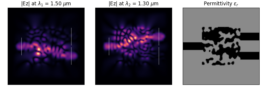
Photonic Inverse Design 2D Problem (Wavelength Demultiplexer).

Problem Description#

Optimize a 2D material distribution (rho) to function as a wavelength demultiplexer, routing wave with lambda1 to output 1 and lambda2 to output 2. The design variables represent material density which is converted to permittivity using filtering and projection.

Design space#

2D tensor rho (num_elems_x, num_elems_y) with values in [0, 1], representing material density. Stored as design_space (gymnasium.spaces.Box).

Objectives#

neg_field_overlap: Combined objective to minimize, defined as penalty - overlap1 * overlap2. Lower is better. This is the value returned by simulate and corresponds to the overlap in the target electrical fields with the desired demultiplexing locations. Note that optimize internally works with a normalized version for stability (penalty - normalized_overlap) and reports history (OptiStep) corresponding to that normalized version. Note: This means comparing the values returned by simulate and optimize directly may not yield similar numbers.

Conditions#

These are designed as user-configurable parameters that alter the problem definition. Default problem parameters that can be overridden via the config dict:

lambda1: The first input wavelength in μm (default: 1.5 μm).
lambda2: The first input wavelength in μm (default: 1.3 μm).
blur_radius: Radius for the density blurring filter (default: 2). Higher values correspond to larger elements, which could possibly be more manufacturable.
num_elems_x: Number of grid cells in x (default: 120).
num_elems_y: Number of grid cells in y (default: 120).

In practice, for the dataset loading, we will keep num_elems_x and num_elems_yto set values for each dataset, such that different resolutions correspond to different independent datasets.

Optimization Parameters#

Note: These are advanced parameters that alter the optimization process – we do not recommend changing these if you are only using the library for benchmarking, as it could make results less reproducible across papers using this problem.)

num_optimization_steps: Total number of optimization steps (default: 300).
step_size: Adam optimizer step size (default: 1e-1).
penalty_weight: Weight for the L2 penalty term (default: 1e-2). Larger values reduce unnecessary material, but may lead to worse performance if too large.
eta: Projection center parameter (default: 0.5). There is little reason to change this.
N_proj: Number of projection applications (default: 1). Increasing this can help make the design more binary.
N_blur: Number of blur applications (default: 1). Increasing this smooths the design more.
save_frame_interval: Interval for saving intermediate design frames during optimization. If > 0, saves a frame every save_frame_interval iterations to the opt_frames/ directory. Default is 0 (disabled).

Internal Constants#

Note: These are not typically changed by users, but provided here for technical reference

dl: Spatial resolution (meters) (default: 40e-9).
Npml: Number of PML cells (default: 20).
epsr_min: Minimum relative permittivity (default: 1.0).
epsr_max: Maximum relative permittivity (default: 12.0).
space_slice: Extra space for source/probe slices (pixels) (default: 8).

Simulator#

The simulation uses the ceviche library’s Finite Difference Frequency Domain (FDFD) solver (fdfd_ez). Optimization uses ceviche.optimizers.adam_optimize with gradients computed via automatic differentiation (autograd).

Dataset#

This problem currently provides one dataset corresponding to resolution of 120x120, are available on the Hugging Face Datasets Hub.

v0#

Fields#

Each dataset contains:

lambda1: The first input wavelength in μm.
lambda2: The second input wavelength in μm.
blur_radius: Radius for the density blurring filter (pixels).
optimal_design: The optimal design density array (shape num_elems_x, num_elems_y).
optimization_history: A list of objective values from the optimization process (negative field overlap, where lower is better) – This is for advanced use.

Creation Method#

To generate a dataset for training, we generate (randomly, uniformly) swept over the following parameters:

\(\lambda_1 \in [0.5\mu m, 1.25\mu m]\) = lambda1 = rng.uniform(low=0.5, high=1.25, size=20) – This corresponds roughly to a portion of the visible spectrum up to near-infrared.
\(\lambda_2 \in [0.75\mu m, 1.5\mu m]\) = lambda2 = rng.uniform(low=0.75, high=1.5, size=20) – This corresponds roughly to a portion of the visible spectrum up to near-infrared.
\(r_{blur}\) = blur_radius = range(0, 5)

Citation#

This problem is directly refactored from the Ceviche Library: https://github.com/fancompute/ceviche and if you use this problem your experiments, you can use the citation below provided by the original library authors:

@article{hughes2019forward,
    title={Forward-Mode Differentiation of Maxwell's Equations},
    author={Hughes, Tyler W and Williamson, Ian AD and Minkov, Momchil and Fan, Shanhui},
    journal={ACS Photonics},
    volume={6},
    number={11},
    pages={3010--3016},
    year={2019},
    publisher={ACS Publications}
}

Lead#

Mark Fuge @markfuge

Photonics2D

Contents